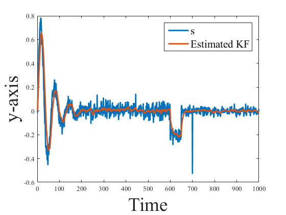
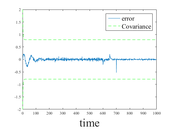
clear
close all
load('signal');

% Process Noise Covariance Declaration
Rww=0.34^2;
% Measurement Noise Covariance Declaration
Rvv=2^2;
%Initial Covariance
P0=4;

%Call function Kalman_Filter
[x,K,P,M_D]= Kalman_Filter(P0,y_s1, Rww, Rvv,1,0.1);

%Plot signal and filtered signal
figure(1)
p1=plot(y_s1,'LineWidth',2);
hold on
p2=plot(x,'LineWidth',2);

ylabel('y-axis','FontSize', 28);
xlabel('Time', 'FontSize',28);
legend({'s','Estimated KF'},'FontSize',16)
set(gca,'FontName','Times');

%Plot the error and the covariance
figure(2)
plot(y_s1(1,:)-x(1,:))
hold on
plot(sqrt(squeeze(P(1,1,:))),'--','Color','G');
plot(-sqrt(squeeze(P(1,1,:))),'--','Color','G');
xlabel('time', 'FontSize',28);
legend({'error','Covariance'},'FontSize',16)
set(gca,'FontName','Times');
Introduction
Confused with the Kalman filter? No worries! I am going to teach you the basics. From now on, you will become an expert. OK, probably not an expert, but you will be able to use it and understand how it works.
The math behind itBefore presenting the Kalman filter equations, it is necessary to first define a state-space model of the system. In this implementation, let's assume that our state vector is $\textbf{x}$ = $[s]$. Where $s$ is a signal acquired from a sensor. This sensor could be an ultrasound measuring distance from a quadcopter, or the voltage in an noisy RC circuit, whatever application you have in mind, you name it, for our general purposes, I'm not going to assign units to $s$. \begin{align*} \textbf{x}(t) &= A\textbf{x}(t-1) + B\textbf{u}(t) + \textbf{w}(t)\\ \textbf{y}(t) &= C\textbf{x}(t) + \textbf{v}(t) \end{align*} The two previous equations represents the system dynamics and the measurement model respectively. Including the state transition matrix $A$, the influence of the control action $B$ (not implemented in our case), the process noise $\textbf{w}$, the observation matrix $C$ and the measurement noise $\textbf{v}$. The process noise is white, Gaussian, with variance $R_{ww}$ and measurement noise is white, Gaussian with variance $R_{vv}$. The standard Kalman filter is comprised of two major components and three intermediary calculations. The two major components are a prediction step and an update step. The update step refines, or corrects, the previous prediction. The three intermediary calculations (innovation, error covariance, and Kalman gain), are necessary for moving from the prediction step to the update step. Below are all the necessary equations for implementing the standard Kalman filter: \begin{align} \label{eq:x_predict} \boldsymbol{\hat{x}}(t|t-1) &= A(t-1)\boldsymbol{\hat{x}}(t-1|t-1) + B\boldsymbol{u}\\ \label{eq:P_predict} \boldsymbol{\hat{P}}(t|t-1) &= A(t-1)\boldsymbol{\hat{P}}(t-1|t-1)A(t-1)^{T}+R_{ww}(t) \end{align} Innovation: \begin{align} \label{eq:e_innovation} \boldsymbol{e}(t) &= \boldsymbol{y}(t) - C(t)\boldsymbol{\hat{x}}(t|t-1)\\ \label{eq:Ree_innovation} R_{ee}(t) &= C(t)\boldsymbol{\hat{P}}(t|t-1)C(t)^{T} + R_{vv}(t)\\ \label{eq:Kalman_gain} \boldsymbol{K}(t) &= \boldsymbol{\hat{P}}(t|t-1)C(t)^{T}R_{ee}(t)^{-1} \end{align} Update: \begin{align} \label{eq:x_update} \boldsymbol{\hat{x}}(t|t) &= \boldsymbol{\hat{x}}(t|t-1)+\boldsymbol{K}(t)\boldsymbol{e}(t)\\ \label{eq:P_update} \boldsymbol{\hat{P}}(t|t) &= (I - \boldsymbol{K}(t)C(t))\boldsymbol{\hat{P}}(t|t-1) \end{align} Is it perfect?The Kalman filter, like any other filter, is susceptible to outliers. An outlier can be understood as a behavior that is not considered in the model. Several mechanism have been proposed, one of them easy to implement is the Mahalanobis Distance (MD). The MD can be easily explained using point $P$ with coordinates $(x,y)$ and a joint distribution of two variables defined by parameters $\mu$, $\sigma_{x}$ and $\sigma_{y}$. The distance is zero if $P=\mu$. The distance increases as $P$ moves away from $\mu$. Evidently, this method can also be used for more than two dimensions. 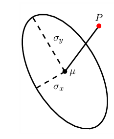
To calculate the MD, one can use the predicted measurement to determine outliers. This error is then defined as follow: given a measurement $\textbf{y} =$ $[y_1$ $y_2$ $...$ $y_N]^{T}$, the MD from this measurement to a group of predicted values with mean $\boldsymbol{\mu} =$ $[\mu_{1}$ $\mu_{2}$ $...$ $\mu_{N}]^{T}$ and innovation covariance matrix $Ree$ is given by \begin{equation} \label{eq:m_dist} M(\textbf{y}) = \sqrt{(\textbf{y}-\boldsymbol{\mu})^{T}Ree^{-1}(\textbf{y}-\boldsymbol{\mu})} \end{equation} The MD can be approximated by the following equation \begin{equation} \label{eq:m_dist_aprox} M({y}) \approx \sum_{i=1}^{N} \left(\frac{{q_{i}}^2}{Ree_{i}}\right)^{1/2} \end{equation} where ${q_{i}=y_{i}-\mu_{i}}$ and $Ree_{i}$ is the $i^{th}$ value along the diagonal of the innovation covariance $Ree$. The program
The Matlab script and the signal can be found below. Also, there is an option to download the files. Make sure to download them all and include them in the same folder (Do not forget the signal.mat). If you are able to run it, you will be able to see the image below. Also, the script allows to make use of the MD, or just use the regular Kalman Filter without outlier rejection.
filter.m
kalman_filter.m
%Kalman Filter with outlier rejection


%function [x,K,P,M_D]= Kalman_Filter(P0, X, Rww, Rvv,MD_act,M_D_val)

%                       Returns:
%                      -x= Filtered Signal
%                      -K=Kalman Gain
%                      -P=Covariance
%                      -M_D=Mahalanbis Distance value

%                       Inputs:
%                      -P0=Initial Covariance (usually high)
%                      -X=Signal
%                      -Rww=Process Noise Covariance
%                      -Rvv=Measurement Noise Covariance
%                      -MD_act= 1-Activaded
%                                0-Desactivaded
%                      -M_D_val= The treshold distance, if MD_act=1.
%                       Otherwise, use 0.

function [x,K,P,M_D]= Kalman_Filter(P0, X, Rww, Rvv,MD_act,M_D_val)


T=length(X);
x=zeros(1,T);
%Transition Matrix
A = [1];
%Measurement Matrix
C = [1];

%Initialization
x0 = 0;
X(1)=x0;
P = zeros(1,1,T);
P(1)=P0;


    for i=2:T

        %prediction
        x(i) = A*x(i-1);
        P(:,:,i) = A*P(:,:,i-1)*A' + Rww;

        %update
        e(:,i) = X(i)-C*x(i);
        Ree(:,:,i) = C*P(:,:,i)*C' + Rvv;
        %Mahalanobis Distance Calculation
        M_D(i)=sqrt(e(:,i)^2)/Ree(:,:,i);

        %1-Use Mahalanobis Distance, 0-Not use Mahalanobis Distance
        if MD_act==1
          if(M_D(i)>=M_D_val)
              x(i)=x(i-1);
              P(:,:,i)= P(:,:,i-1);
          else
              K = P(:,:,i)*C'*(Ree(:,:,i)^-1);
              x(:,i) = x(:,i) + K*e(:,i);
              P(:,:,i) = (1-K*C)*P(:,:,i);
          end
        else
          K = P(:,:,i)*C'*(Ree(:,:,i)^-1);
          x(:,i) = x(:,i) + K*e(:,i);
          P(:,:,i) = (1-K*C)*P(:,:,i);
        end
    end
end
Are the results right?
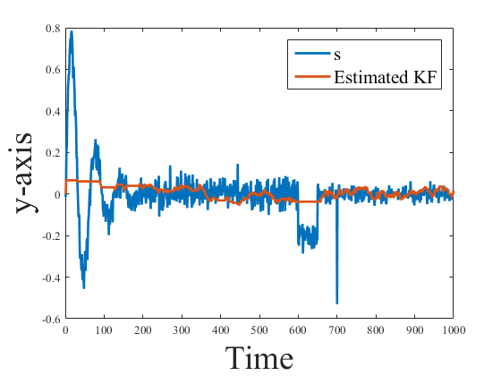
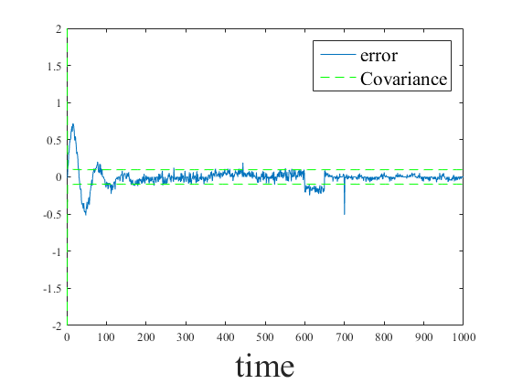
For those that have not noticed, I am doing estimation with a KF that uses a first order model. But, it turns out that the system seems to be a second order model. If you see the covariance, it seems a little bit high for this purpose. Also, around the time 600 and 650, the sensor suffers a shock that the filter could not estimate properly. However, the MD was able to account for the spike around the 700 time iteration. A better model could have given better results. Also different parameters for the measurement and noise covariance causes other results.
In the previous graph we were able to ignore the two oscillations, the shock and the spike. These errors are common in any sensor. Try to think of the process and measurement noise covariances as weights, or trust values. Also the results involves that you have a deep knowledge of the physics behind your system, this will help you to choose the best parameters, tuning a KF is considered an arcane and dark science (not really, but it involves a lot of knowledge from you side).
Conclusions
The Kalman Filter is by far one of the most useful tools in signal processing. It has been applied in fields such as robotics, computer vision, biology, econometrics and many more. The Kalman Filter is widely use for its ease of implementation.
Other well known estimator is the Particle Filter, that I will cover in other post. Also, we will keep adding more functions to the Matlab script, that will allow to apply different models to produce better and more accurate estimations. If you have any question, make sure to leave a comment.
0 Comments
Leave a Reply. |
About meEvery venture in an unknown territory is exciting to me. I ended up working with autonomous robots using knowledge from fields such as; computer vision, Bayesian estimation, control theory, neural networks, and SLAM. I have always been fascinated by aerial and ground mobile vehicles. Thankfully I had the chance to work on algorithms that bring them to life. 
Archives |
||||||||||